I don't know about others but when I started digging into machine-learning I had some problems understanding bias-variance until I found a nice target shooting analogy.
Target
Out little target chart :) with some params.
  import numpy as np
  color = hue(1)
  size = 50
  p = plot([], figsize=7)
  p += plot(circle((0,0), 1))
  p += plot(circle((0,0), 3))
  p += plot(circle((0,0), 6))
  p
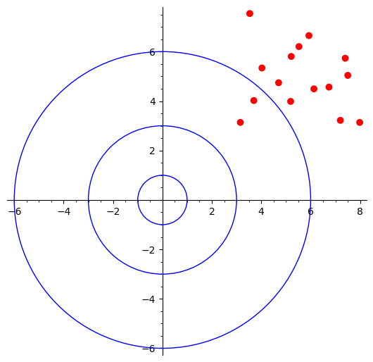
High bias and high variance
Worst-case scenario where hits are all over the places (high variance) and far away from the center of target, top-right skewed (high bias).
  variance = 5
  bias = 3
  samples = variance * np.random.random_sample((15, 2)) + bias
  hbhv = p + plot(point(samples, rgbcolor=color, size=size))
  hbhv
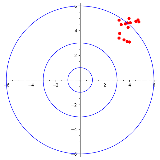
High bias and low variance
This time the shots are focused (low variance) within a small area that is still far away (high bias) from the target.
  variance = 2
  bias = 3
  samples = variance * np.random.random_sample((15, 2)) + bias
  hblv = p + plot(point(samples, rgbcolor=color, size=size))
  hblv
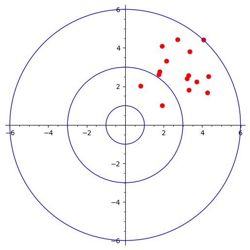
Low bias and high variance
This time all hots are closer to center (low bias) but still spread all over the places (high variance).
  variance = 4
  bias = 0.5
  samples = variance * np.random.random_sample((15, 2)) + bias
  lbhv = p + plot(point(samples, rgbcolor=color, size=size))
  lbhv
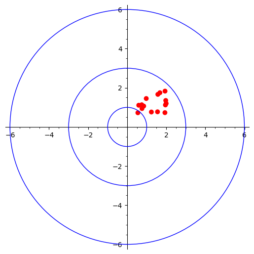
Low bias and low variance
The best case scenario, focused (low variance) and very close to center (low bias).
  variance = 1.5
  bias = 0.5
  samples = variance * np.random.random_sample((15, 2)) + bias
  lblv = p + plot(point(samples, rgbcolor=color, size=size))
  lblv
Happy shooting!!!