Historical volatility -

Historical volatility (also called realized volatility) measures how far the normal standard deviation is from expected mean, over a given period of time.

OK, OK, it ain't explain shit … what is it?

Get data

We are going to use CryptoCompare's FREE API and fetch daily OHLC prices for BTCUSD.

  import pandas as pd

  url = "https://min-api.cryptocompare.com/data/v2/histoday?fsym=BTC&tsym=USD&limit=100"
  response = pd.read_json(url, convert_dates=['time'])
  df = pd.DataFrame(response["Data"]["Data"], columns=['time', 'open', 'high', 'low', 'close'])
  print(df.tail())

           time      open      high       low     close
96   1616112000  57643.32  59453.32  56283.37  58060.21
97   1616198400  58060.21  59911.70  57837.79  58101.34
98   1616284800  58101.34  58621.34  55635.61  57374.95
99   1616371200  57374.95  58431.44  53795.78  54095.36
100  1616457600  54095.36  55455.64  52984.36  55141.96

Transform data

Time column seems to be the returned as timestamp but we want to work with date type instead, let's cast it.

  df['time'] = df['time'].astype('datetime64[s]')
  print(df.tail())

          time      open      high       low     close
96  2021-03-19  57643.32  59453.32  56283.37  58060.21
97  2021-03-20  58060.21  59911.70  57837.79  58101.34
98  2021-03-21  58101.34  58621.34  55635.61  57374.95
99  2021-03-22  57374.95  58431.44  53795.78  54095.36
100 2021-03-23  54095.36  55455.64  52984.36  55141.96

Return

Why we use log returns instead of simple returns is a longer story but you can see it as simple rate vs. continuously compounded rate.

Detalied info in returns, risk-adjusted ratios, metrics and interest-rate blog posts.

\[ \textcolor{blue} { r_i = \log{\frac{x_i}{x_{i-1}}} = \log({x_i}) - \log{(x_{i-1})} } \]

  import numpy as np

  df = df.assign(prev_close=df.close.shift(1))
  df = df.assign(logr=np.log(df.close / df.prev_close))
  print(df.tail())

          time      open      high       low     close  prev_close      logr
96  2021-03-19  57643.32  59453.32  56283.37  58060.21    57643.32  0.007206
97  2021-03-20  58060.21  59911.70  57837.79  58101.34    58060.21  0.000708
98  2021-03-21  58101.34  58621.34  55635.61  57374.95    58101.34 -0.012581
99  2021-03-22  57374.95  58431.44  53795.78  54095.36    57374.95 -0.058859
100 2021-03-23  54095.36  55455.64  52984.36  55141.96    54095.36  0.019163

Variance

Variance (σ² - sigma squared) is the average of squared distances from the mean (μ - mu).

\[ \textcolor{blue} { \sigma^2 = \frac{\sum_{i=1}^{N} (r_i - \mu)^2}{N} } \]

  n = df['logr'].size - 1
  print("Total " + str(n) + " samples in dataset")

  mu = df['logr'].mean()
  print(mu)

  def squared_distance(x, m):
     return (x - m)**2
  variance = df['logr'].apply(squared_distance, args=(mu,)).sum() / n
  print(variance)

Total 100 samples in dataset
0.010566139516163857
0.0022171923333002158

Volatility

Volatility (σ - sigma) is as simple as square root of variance. Volatility is also known as 1st standard deviation of a normal distribution and we know that log returns are normally distributed.

\[ \textcolor{blue} { \sigma = \sqrt{\frac{\sum_{i=1}^{N} (r_i - \mu)^2}{N}} } \]

  vol = np.sqrt(variance)
  print(vol)

  std = df['logr'].std()
  print(std)

0.04708707182762818
0.04732428779659303

Most of the time we will work with annualized volatility that is daily volatility * square root of trading days where trading days is 365 for crypto markets.

  annualized_vol = vol * np.sqrt(365)
  print(annualized_vol)

0.8995972441346064

Rolling volatility

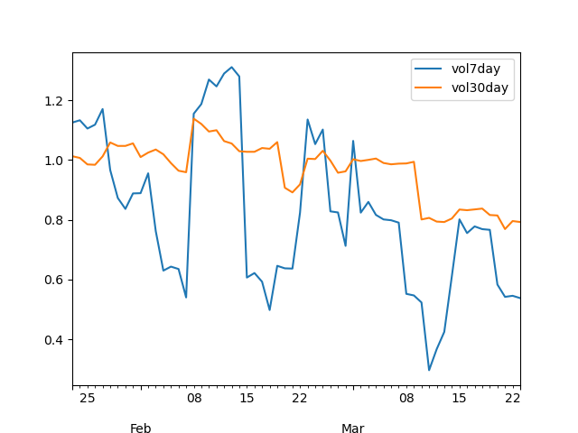
This is just the historical volatility average for a past rolling window, e.g. 7-day, 30-day, etc.

  def volatility(w, n):
     mu = w.mean()
     variance = w.apply(squared_distance, args=(mu,)).sum() * 365 / n
     return np.sqrt(variance)
  df = df.assign(vol7day=df.logr.rolling(7).apply(volatility, args=(7,)))
  df = df.assign(vol30day=df.logr.rolling(30).apply(volatility, args=(30,)))
  print(df.loc[:, ['time', 'vol7day', 'vol30day']].tail())

          time   vol7day  vol30day
96  2021-03-19  0.766401  0.815991
97  2021-03-20  0.583027  0.814464
98  2021-03-21  0.541779  0.768962
99  2021-03-22  0.545397  0.795786
100 2021-03-23  0.537617  0.792567

And here are the 7-day vs. 30-day rolling volatility graphs:

  import matplotlib.pyplot as plt
  filename = 'hv-rolling.png'
  plt.figure(figsize=(8, 6))
  df[-60:].plot(x='time', y=['vol7day','vol30day'])
  plt.savefig(filename)
  filename

/img/hv/hv-rolling.png

Volatility models

Close-close

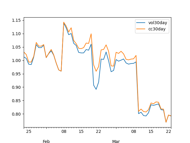
Close-close historical volatility model is quite similar to classic model calculated above with 2 main differences:

we assume mean = 0, here no distance from the mean sub, only the squared log returns
we calculate annualized volatility, mind the 365 term under the square root

\[ \textcolor{blue} { \sigma_{cc} = \sqrt{\frac{\sum_{i=1}^{N} \ln{\frac{r_i}{r_{i-1}}}^2 * 365 }{N}} } \]

  def squared_log(r):
    return r**2
  def closeclose(w, n):
    var = w.apply(squared_log).sum() * 365 / n
    return np.sqrt(var)
  df = df.assign(cc30day=df.logr.rolling(30).apply(closeclose, args=(30,)))
  print(df.loc[:, ['time', 'logr', 'cc30day']].tail())

          time      logr   cc30day
96  2021-03-19  0.007206  0.818845
97  2021-03-20  0.000708  0.817973
98  2021-03-21 -0.012581  0.769133
99  2021-03-22 -0.058859  0.796060
100 2021-03-23  0.019163  0.793004

Close-close vs. classic 30-day volatility, quite similar with the other one.

  filename = 'hv-closeclose.png'
  df[-60:].plot(x='time', y=['vol30day', 'cc30day'])
  plt.savefig(filename)
  filename

/img/hv/hv-closeclose.png

Parkinson

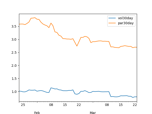
Close-close model uses today's close vs. yesterday's close and ignores a lot of intraday volatility but Parkinson model tries to solve the problem using high (hᵢ) and low (lᵢ) prices.

\[ \textcolor{blue} { \sigma_{pa} = \sqrt{\frac{\sum_{i=1}^{N} \ln{\frac{h_i}{l_i}}^2 * 365 }{N * 4 * \ln2}} } \]

  def parkinson(w, n):
    var = w.apply(squared_log).sum() * 365 / n * 4 * np.log(2)
    return np.sqrt(var)
  df = df.assign(hllogr=np.log(df.high / df.low))
  df = df.assign(par30day=df.hllogr.rolling(30).apply(parkinson, args=(30,)))
  print(df.loc[:, ['time', 'hllogr', 'par30day']].tail())

          time    hllogr  par30day
96  2021-03-19  0.054792  2.729470
97  2021-03-20  0.035229  2.730649
98  2021-03-21  0.052275  2.680251
99  2021-03-22  0.082659  2.699996
100 2021-03-23  0.045587  2.697506

Parkinson vs. classic 30-day volatility, huge differences since high-low movements are larger than open-close.

  filename = 'hv-parkinson.png'
  df[-60:].plot(x='time', y=['vol30day', 'par30day'])
  plt.savefig(filename)
  filename

/img/hv/hv-parkinson.png

Garman-Klass

To improve the Parkinson model, GKs use both close-open and high-low prices.

\[ \textcolor{blue} { \sigma_{gk} = \sqrt{\frac{365}{N}} * \sqrt{\sum_{i=1}^{N} \frac{\ln{\frac{h_i}{l_i}}^2}{2} - (2*\ln2-1) * \sum_{i=N}^{N} \ln{\frac{c_i}{o_i}}^2 } } \]

Rogers-Satchel

Then comes RS and

\[ \textcolor{blue} { \sigma_{rs} = \sqrt{\frac{365}{N}} * \sqrt{\sum_{i=N}^{N} \ln{\frac{h_i}{c_i}} \ln{\frac{h_i}{o_i}} + \ln{\frac{l_i}{c_i}} \ln{\frac{l_i}{o_i}} } } \]

Yang-Zang

And finally the YZ model that takes into account both jumps and drift.

\[ \textcolor{blue} { \sigma_{yz} = \sqrt{365} * \sqrt{ \sigma_{close-to-open}^2 + k*\sigma_{open-to-close}^2 + (1-k)* \sigma_{rs}^2 } } \]

where: \[ \textcolor{blue} { k = \frac{0.34}{1.34 + \frac{N+1}{N-1}} } \]

\[ \textcolor{blue} { \sigma_{close-to-open}^2 = \frac{1}{N-1} * \sum_{i=N}^{N} { [\ln(\frac{o_i}{c_{i-1}})-\overline{\ln(\frac{o_i}{c_{i-1}})}]^2 } } \]

\[ \textcolor{blue} { \sigma_{open-to-close}^2 = \frac{1}{N-1} * \sum_{i=N}^{N} { [\ln(\frac{c_i}{o_i})-\overline{\ln(\frac{o_i}{c_i})}]^2 } } \]

Daunting huh? Not really, just formulas with multiple terms for a more accurate estimation, the underlying volatility concepts stay the same.

References