Overview
Big-O notation or Big Omicron (e.g. Ο(n)) also called "asymptotic growth" notation is used to represent the worst-case scenario (the upper bound) for a given algorithm.
There is also Big Omega (e.g. Ω(n)) the lower bound and Big Theta (e.g. Θ(n)) both upper and lower bound of an algorithm.
Complexity of an algorithm (the number of operations/the run time) is directly proportional with input size n.
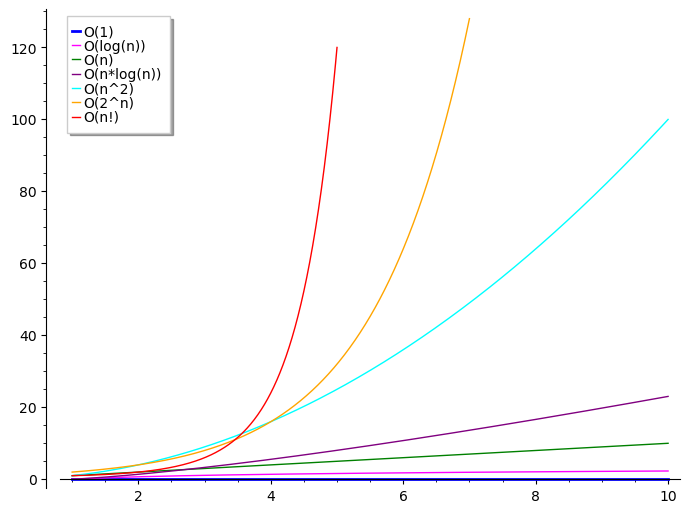
Here is the graph of the most common growth functions:
p = plot([], figsize=7)
p += plot(0, (1, 10), color='blue', legend_label='O(1)', thickness=2)
p += plot(log(x), (1, 10), color='magenta', legend_label='O(log(n))')
p += plot(x, (1, 10), color='green', legend_label='O(n)')
p += plot(x * log(x), (1, 10), color='purple', legend_label='O(n*log(n))')
p += plot(x^2, (1, 10), color='cyan', legend_label='O(n^2)')
p += plot(2^x, (1, 7), color='orange', legend_label='O(2^n)')
p += plot(factorial(x), (1, 5), color='red', legend_label='O(n!)')
p

You can easily see the red line is exploding to the upside when x>4 while the magenta line looks almost horizontal but let's have a closer look at each individual function.
O(1)
Constant complexity - the number of operations is always the same regardless the size of the input (blue line)
p = plot([], figsize=7)
p += plot(0, (1, 10), color='blue', legend_label='O(1)', thickness=2)
p
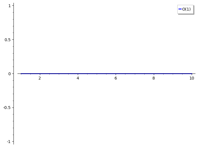
Examples: array access, list append, queue push/pop, hash table insert/delete
O(log n)
Logarithmic complexity - the number of computations is increased by a log of the input (magenta line)
p = plot([], figsize=7)
p += plot(0, (1, 10), color='blue', legend_label='O(1)', thickness=2)
p += plot(log(x), (1, 10), color='magenta', legend_label='O(log(n))')
p
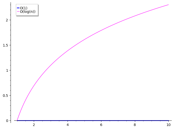
Examples: insert/search/delete operations on tree-like structures (b-tree, red-black)
O(n)
Linear complexity - increases linearly with the input size (green line)
p = plot([], figsize=7)
p += plot(0, (1, 10), color='blue', legend_label='O(1)', thickness=2)
p += plot(log(x), (1, 10), color='magenta', legend_label='O(log(n))')
p += plot(x, (1, 10), color='green', legend_label='O(n)')
p
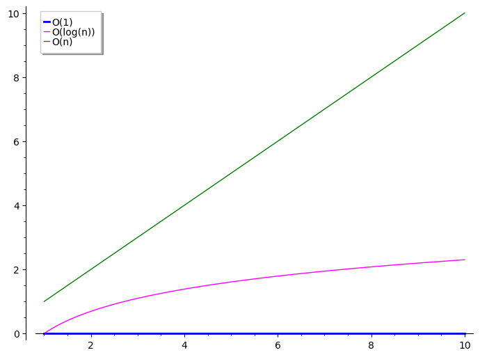
Examples: unordered search in array/queue/stack/list or access in queue/list
O(n * log n)
Log linear complexity - product of linear and logarithmic (purple line)
p = plot([], figsize=7)
p += plot(0, (1, 10), color='blue', legend_label='O(1)', thickness=2)
p += plot(log(x), (1, 10), color='magenta', legend_label='O(log(n))')
p += plot(x, (1, 10), color='green', legend_label='O(n)')
p += plot(x * log(x), (1, 10), color='purple', legend_label='O(n*log(n))')
p
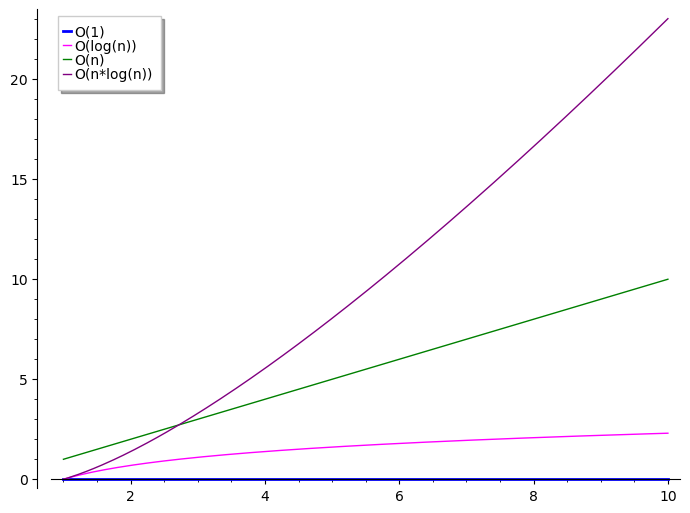
Examples: a few (merge sort, quick sort) array sorting algorithms
O(n^c)
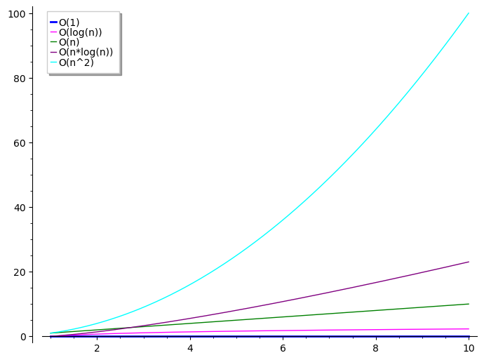
Polynomial complexity - input size as base (cyan line)
Any algorithm that has a polynomial complexity is executed in polynomial time. On graph we only draw O(n^2) (a special case where c=2 which is called quadratic complexity) but the growth rate is a lot bigger, see how the other lines are flattened.
p = plot([], figsize=7)
p += plot(0, (1, 10), color='blue', legend_label='O(1)', thickness=2)
p += plot(log(x), (1, 10), color='magenta', legend_label='O(log(n))')
p += plot(x, (1, 10), color='green', legend_label='O(n)')
p += plot(x * log(x), (1, 10), color='purple', legend_label='O(n*log(n))')
p += plot(x^2, (1, 10), color='cyan', legend_label='O(n^2)')
p
Examples: many (bubble, insertion, selection, tree) array sorting algorithms
O(c^n)
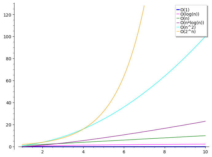
Exponential complexity - input size as exponent and constant c > 1 (orange line)
p = plot([], figsize=7)
p += plot(0, (1, 10), color='blue', legend_label='O(1)', thickness=2)
p += plot(log(x), (1, 10), color='magenta', legend_label='O(log(n))')
p += plot(x, (1, 10), color='green', legend_label='O(n)')
p += plot(x * log(x), (1, 10), color='purple', legend_label='O(n*log(n))')
p += plot(x^2, (1, 10), color='cyan', legend_label='O(n^2)')
p += plot(2^x, (1, 7), color='orange', legend_label='O(2^n)')
p
Examples: recursive algorithms like Fibonacci numbers calculation
O(n!)
Factorial complexity - astronomic growth rate
p = plot([], figsize=7)
p += plot(0, (1, 10), color='blue', legend_label='O(1)', thickness=2)
p += plot(log(x), (1, 10), color='magenta', legend_label='O(log(n))')
p += plot(x, (1, 10), color='green', legend_label='O(n)')
p += plot(x * log(x), (1, 10), color='purple', legend_label='O(n*log(n))')
p += plot(x^2, (1, 10), color='cyan', legend_label='O(n^2)')
p += plot(2^x, (1, 7), color='orange', legend_label='O(2^n)')
p += plot(factorial(x), (1, 5), color='red', legend_label='O(n!)')
p
Examples: classical traveling salesman problem - given n towns find the shortest route that visit every town. This is hard problem that cannot be solved in polynomials time O(n^c), it's a factorial (combinatorial) order problem.
For n = 60 we have:
factorial(60) > 10^80True
where 10^80 is the number of atoms in visible universe so you better think twice about this growth rate.
If somebody asks what is the growth rate of your business, you can show off by saying that it is factorial. ;)
References
- https://en.wikipedia.org/wiki/Big_O_notation
- https://en.wikipedia.org/wiki/Computational_complexity_theory
- https://en.wikipedia.org/wiki/Master_theorem_(analysis_of_algorithms)
- https://stackoverflow.com/questions/13467674/determining-complexity-for-recursive-functions-big-o-notation/43991156#43991156
Happy factoring!!!