Black-Scholes formula

Black-Scholes formula… maybe not as important and well-known as compounding interest-rate but still the most famous formula among options traders. Here are the formulas that you will find in financial books.

Intuition

\[ d1 = \frac{\ln{\frac{\textcolor{blue}{S}}{\textcolor{cyan}{K}}} + (r + \frac{\textcolor{lime}{\sigma}^2}{2}) * \textcolor{magenta}{t}}{\textcolor{lime}{\sigma}*\sqrt{\textcolor{magenta}{t}}} \\ d2 = \frac{\ln{\frac{\textcolor{blue}{S}}{\textcolor{cyan}{K}}} + (r - \frac{\textcolor{lime}{\sigma}^2}{2}) * \textcolor{magenta}{t}}{\textcolor{lime}{\sigma}*\sqrt{\textcolor{magenta}{t}}} \]

\[ \textcolor{green} {C} = N(d1) * \textcolor{blue}{S} - N(d2) * \textcolor{cyan}{K} * e^{-r*\textcolor{magenta}{t}} \]

\[ \textcolor{red} {P} = N(-d2) * \textcolor{cyan}{K} * e^{-r*\textcolor{magenta}{t}} - N(-d1) * \textcolor{blue}{S} \]

where:

C - price of an European Call options
P - price of an European Put options
N - cumulative distribution function (CDF)
S - Spot price of the underlying asset
K - striKe price of option
t - time to expiraTion (in years)
σ - sigma - standard deviation of log returns (volatility)
σ² - squared deviation (variance)

Scary? not really… let's put d1 and d2 terms aside for now and try to understand the call/put price formulas.

We know the discounted interest-rate formula, details and proof in this blog post.

\[ \color{blue} D = C * e^{-r*t} \]

where

C - the compounding value (forward/future price) after t time and D is present value (current price); or put the it other way around, D is the discounted value of C.
D - present value (discounted value) of the strike price K

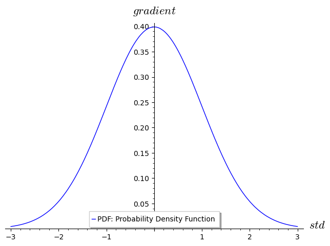
What about N( ) thing? First thing first, let's have a look at Gaussian distribution (also called normal distribution) with 1 standard deviation (σ = 1) and 0 mean (μ = 0)

  G = RealDistribution('gaussian', 1)

  PDF = lambda x: G.distribution_function(x)
  plot(PDF, (x, -3, 3), legend_label='PDF: Probability Density Function', axes_labels=['$std$', '$gradient$'])

/img/blackscholes/pdf.png

Since PDF is probability density function we are dealing with areas of probabilities, in simple terms, the area to the left of the mean has 50% probability.

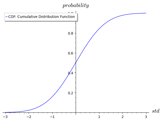
  CDF = lambda x: G.cum_distribution_function(x)
  plot(CDF, (x, -3, 3), legend_label='CDF: Cumulative Distribution Function', axes_labels=['$std$', '$probability$'])

/img/blackscholes/cdf.png

CDF is called cumulative distribution function which is the probability of a random variable X to be less than a given point x.

Without going into details, the relation between the two is that, we can integrate the density function and find the cumulative function

\[ \int_{-\infty}^x PDF(x) \, \mathrm{d}x = CDF(x) \]

and vice-versa, we differentiate the cumulative function and find the density function.

\[ \frac{\mathrm{d} \, CDF(x)}{\mathrm{d}x} = PDF(x) \]

Finally, since our N( ) function is a CDF it means that it is 0 < N( ) < 1, in other words it is a weight (a scaling factor).

With this new knowledge, let's change the call/put price formulas to:

\[ \textcolor{green} {C} = N(d1) * \textcolor{blue}{S} - N(d2) * \textcolor{cyan}{D} \]

\[ \textcolor{red} {P} = N(-d2) * \textcolor{cyan}{D} - N(-d1) * \textcolor{blue}{S} \]

In conclusion:

the price for a CALL option can be viewed as:

profit/loss amount: a scaling factor times the underlying price at expiry
minus
amount that we pay: scaling factor times discounted value of the strike price now

and a PUT options as:

amount that we pay - scaling factor times discounted value of the strike price now
minus
profit/loss amount - scaling factor times the underlying spot price at expiration

Implementation

In Python/Sagemath it looks like this:

  from math import log, sqrt, pi, exp

  def d1(s, k, t, r, iv):
      return(log(s/k) + (r+iv**2/2)*t) / iv*sqrt(t)
  def d2(s, k, t, r, iv):
      return d1(s,k,t,r,iv) - iv*sqrt(t)

  def D(k, r, t):
      return k * exp(-r*t)
  def N(d):
      return CDF(d)

  def call_price(s, k, t, r, iv):
      return N(d1(s,k,t,r,iv)) * s - N(d2(s,k,t,r,iv)) * D(k,r,t)
  def put_price(s, k, t, r, iv):
      return N(-d2(s,k,t,r,iv)) * D(k,r,t) - N(-d1(s,k,t,r,iv)) * s

Call price:

  s = 1330
  k = 1280
  t = (10 + 17/24) / 365
  r = 0.01
  iv = 1.34
  print(call_price(s, k, t, r, iv))

141.6089647684081

Put price:

  s = 33760
  k = 34000
  t = (10 + 17/24) / 365
  r = 0.01
  iv = 1.10
  print(put_price(s, k, t, r, iv))

2655.0941969718187

Implied volatility

We can do it the other way around as well and recursively find the implied volatility for a given price.

Call IV:

  def call_iv(p, iv=1.30, step=0.01):
      ip = call_price(s, k, t, r, iv)
      if ip > p:
          return iv;
      else:
          return call_iv(p, iv + step)

  print(call_iv(141))

1.34000000000000

Put IV:

  def put_iv(p, iv=1.00, step=0.01):
      ip = put_price(s, k, t, r, iv)
      if ip > p:
          return iv;
      else:
          return put_iv(p, iv + step)

  print(put_iv(2660))

1.11000000000000

References

trading options put call black-scholes volatility python