The easiest way to understand Elliptic Curve (EC), point addition, scalar multiplication and trapdoor function; explained with simple graphs and animations.

1. Abstract

What the heck is an elliptic curve?
A plane algebraic curve defined by an equation of this form: y² = x³ + a*x + b
Why are elliptic curves important in cryptography?
Because elliptic curve scalar multiplication is a trapdoor function
How does scalar multiplication works?
Scalar/point multiplication is defined as repeated addition of a point to itself
How does point addition works then?
If we draw a line passing thru elliptic curve points (or draw a tangent to a single point) it will intersect another point on the curve and the inverse of this intersection point if the result of point addition

Since a picture is worth a thousand words then the following elliptic curve point addition/multiplication animation has 33 frames and is worth a lot more, do the math.

Given an elliptic curve E a point on elliptic curve G (called the generator) and a private key k we can calculate the public key P where P = k * G.

The whole idea behind elliptic curves cryptography is that point addition (multiplication) is a trapdoor function which means that given G and P points it is infeasible to find the private key k.

Keep reading if you are interested to understand more about the subject.

2. A bit of math

Before jumping into elliptic curves math lets do a recap of basic algebraic structures.

Simple structures - no binary operation

Set - collection of distinct objects
Unary - a set and an unary operation over set

Group-like structures - one binary operation

Magma - a set with a closed binary operation
Semigroup - an associative magma
Monoid - a semigroup with identity element
Group - a monoid with unary operation (inverse)
1. Abelian group - a group whose binary operation is also commutative

Takeaway - group’s properties:

is a collection of objects/numbers
has a closed binary operation
is associative
has an identity element
has inverse elements
might be commutative

3. Examples of elliptic curves

As always, I am going to leverage the power of the trinity (Emacs, Orgmode, Python/Sagemath) to draw a few explanatory graphs.

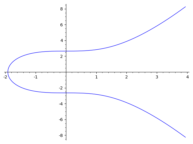
Let’s start with a simple elliptic curve with the following parameters: a=0, b=7.

E = EllipticCurve([0, 7])
E.plot()

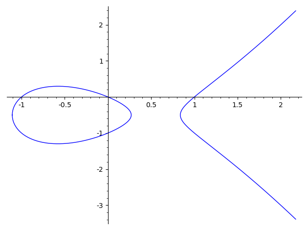
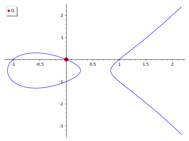
Not very interesting … let’s pick a fancy one with parameters: a=-1, b=0 (don’t worry about the first 3 params)

E = EllipticCurve([0,0,1,-1,0])
E.plot()

4. Points on elliptic curve

Generator point

We can see that origin seems to be a point on our curve, let’s check it out.

E = EllipticCurve([0,0,1,-1,0])
G = E([0, 0])
g = E.plot()
g += G.plot(legend_label="G", color="red", pointsize=100)
g.show()

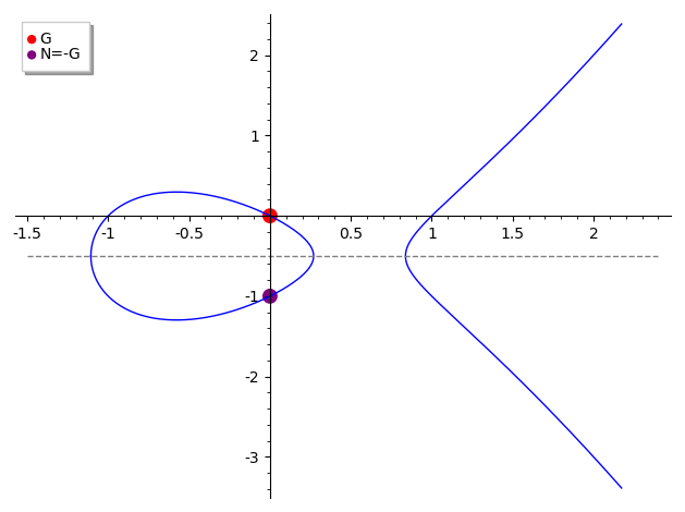
Inverse point

According to property #5, each point has an inverse point. What is the inverse operation with respect to addition? It’s negation.

E = EllipticCurve([0,0,1,-1,0])
G = E([0, 0])
N = -G
g = E.plot()
g += G.plot(legend_label="G", color="red", pointsize=100)
g += N.plot(legend_label="N=-G", color="purple", pointsize=100)
g += line([(-1.5, -0.50), (2.4, -0.50)], color="gray", linestyle="dashed")
g.show()

Identity point

According to property #4 we have an identity element. What is the result of G - G? it is called point at infinity or identity I and satisfy the equation G + I = G. This is like 0 in arithmetic where 3 + 0 = 3.

Unfortunately I can’t draw it on the graph but you can imagine a vertical line passing thru G and -G points that “intersects” the curve in point at infinity.

One thing to remember is that our generator point above is (0, 0) but that is just a regular point on elliptic curve, nothing special about it.

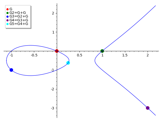
Closed points

Property #2 tells us that binary operation has to be closed, lets see what this means.

Adding the point G to itself (doubling) we can see that resulting point is also on the curve.

If we keep adding more G points we figure out that all points are on the curve and this gives us the closed property of the elliptic curves addition.

E = EllipticCurve([0,0,1,-1,0])
G = E([0, 0])
G2 = G + G
G3 = G2 + G
G4 = G3 + G
G5 = G4 + G
g = E.plot()
g += G.plot(legend_label="G", color="red", pointsize=100)
g += G2.plot(legend_label="G2=G+G", color="green", pointsize=100)
g += G3.plot(legend_label="G3=G2+G", color="blue", pointsize=100)
g += G4.plot(legend_label="G4=G3+G", color="purple", pointsize=100)
g += G5.plot(legend_label="G5=G4+G", color="cyan", pointsize=100)
g.show()

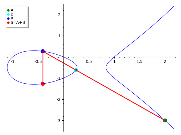
5. Elliptic curve addition

Geometrically, the main rule to add two points on elliptic curve is to draw a line passing thru those points that will intersect the curve in another point and the inverse of this intersection point if the result of point addition. This is all, of course there are a few edge cases to this rule (like A = -B or A == B) but we will keep things simple and ignore the edge cases for now.

E = EllipticCurve([0,0,1,-1,0])
G = E([0, 0])
A = 4 * G
B = 5 * G
S = A + B
X = -S
g = E.plot()
g += A.plot(legend_label="A", color="green", pointsize=100)
g += B.plot(legend_label="B", color="cyan", pointsize=100)
g += X.plot(legend_label="X", color="blue", pointsize=100)
g += S.plot(legend_label="S=A+B", color="red", pointsize=100)
g += line([A.xy(), B.xy(), X.xy()], color="red", thickness=2)
g += line([X.xy(), S.xy()], color="red", thickness=2)
g.show()

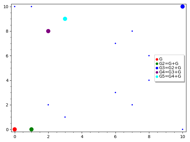
6. Elliptic curve over finite fields

What we’ve seen so far are elliptic curves over rational numbers but what is really used in cryptography are elliptic curves over finite fields.

How does a elliptic curve over finite field looks like?
Well, I am afraid you won’t like the graph because elliptic curves defined over finite fields get cut off and are not intelligible to humans

And the nice thing about this is that all the elliptic curve’s properties are preserved on finite fields as well and point addition / scalar multiplication works as expected.

F = FiniteField(11)
E = EllipticCurve(F, [0,0,1,-1,0])
G = E([0, 0])
G2 = G + G
G3 = G2 + G
G4 = G3 + G
G5 = G4 + G
g = E.plot()
g += G.plot(legend_label="G", color="red", pointsize=100)
g += G2.plot(legend_label="G2=G+G", color="green", pointsize=100)
g += G3.plot(legend_label="G3=G2+G", color="blue", pointsize=100)
g += G4.plot(legend_label="G4=G3+G", color="purple", pointsize=100)
g += G5.plot(legend_label="G5=G4+G", color="cyan", pointsize=100)
g.show(frame=True, axes=False)

Elliptic curves

Cryptography